Insert a blank sheet into the workbook and add hyperlinks to the sheets you need using the command Insert - Hyperlink. In the window that opens, select the option on the left Place in document and set the external text display and the address of the cell where the link will lead:
For convenience, you can also create backlinks on all sheets of your book, which will lead back to the table of contents. In order not to have to manually create hyperlinks and then copy them to each sheet, it is better to use another method - the function HYPERLINK. We select all the sheets in the book where we want to add a backlink (you can use the keys to mass select sheets Shift and/or Ctrl) and in any suitable cell we enter a function of the following form:
This function will create a hyperlink in the current cell on all selected sheets with the text “Back to Table of Contents”, clicking on which will return the user to the sheet Table of contents.
Method 2: Dynamic table of contents using formulas
This, although slightly exotic, is a very beautiful and convenient way to create an automatic table of contents for your book. Exotic - because it uses an undocumented XLM feature GET.WORKBOOK, left by the developers for compatibility with older versions of Excel. This function dumps a list of all sheets in the current workbook into a given variable, from which we can then extract them and use them in our table of contents.
Open Name Manager on the tab Formulas (Formulas – Name Manager) and create a new named range called, let's say Table of contents. In field Range (Reference) enter this formula:

GET.WORK.BOOK(1)
=GET.WORKBOOK(1)
Now in the variable Table of contents contains our searched names. To extract them from there to the sheet, you can use the function INDEX, which “pulls out” elements from the array by their number:
Function ROW gives the current row number and, in this case, is needed only to avoid manually creating a separate column with the serial numbers of the elements being extracted (1,2,3...). Thus, in cell A1 we will have the name of the first sheet, in A2 - the name of the second, etc.

Not bad. However, as you can see, the function returns not only the sheet name, but also the workbook name, which we do not need. To remove it, we use the functions REPLACE (SUBST) And FIND, which will find the closing square bracket character (]) and replace all text up to and including that character with the empty string (""). Let's open it again Name Manager from tab Formulas (Formulas - Name Manager), double click to open the created range Table of contents and change its formula:
=SUBST(GET.WORKBOOK(1);1;FIND("]";GET.WORKBOOK(1));"")
Now our list of sheets will look much better:

A small side complication is that our formula is in a named range Table of contents will be recalculated only when entered, or when the book is forced to recalculate by pressing a key combination Ctrl+Alt+F9. To get around this unpleasant moment, let’s add a small “tail” to our formula:
REPLACE(GET.WORKBOOK(1);1;FIND("]";GET.WORKBOOK(1));"") &T(TDATE())=SUBST(GET.WORKBOOK(1);1;FIND("]";GET.WORKBOOK(1));"")&T(NOW())
Function TDATE (NOW) gives the current date (with time), and the function T turns that date into an empty text string, which is then concatenated to our sheet name using the concatenation operator (&). Those. the sheet name does not actually change, but since the function TDATE is recalculated and produces a new time and date for any change in the sheet, then the rest of our formula will be forced to recalculate too and - as a result - the names of the sheets will be constantly updated.
To hide errors #REFERENCE (#REF), which will appear if we copy our formula with the function INDEX for more cells than we have sheets, we can use the function IFERROR which catches any errors and replaces them with the empty string (""):

And finally, to add “live” hyperlinks to sheet names for quick navigation, you can use the same function HYPERLINK, which will form the address for the transition from the sheet name:

Method 3. Macro
And finally, you can use a simple macro to create a table of contents. True, you will have to run it every time the structure of the book changes - unlike Method 2, the macro itself does not track them.
Open the Visual Basic Editor by clicking Alt+F11 or by selecting (in older versions of Excel) from the menu Tools - Macro - Visual Basic Editor(Tools - Macro - Visual Basic Editor) . In the editor window that opens, create a new empty module (menu Insert - Module ) and copy the text of this macro there:
Sub SheetList()
Dim sheet As Worksheet
Dim cell As Range
With ActiveWorkbook
For Each sheet In ActiveWorkbook.Worksheets
Set cell = Worksheets(1).Cells(sheet.Index, 1)
.Worksheets(1).Hyperlinks.Add anchor:=cell, Address:="", SubAddress:=""" & sheet.Name & """ & "!A1"
cell.Formula = sheet.Name
Next
End With
End Sub
Close the Visual Ba Editor sic and return to Excel. Add a blank sheet to the book and place it first. Then clickAlt+F8or open the menuTools - Macro - Macros. Find the macro you created thereSheetListand run it. The macro will create a list of hyperlinks with sheet names on the first sheet of the workbook. Clicking on any of them will take you to the desired sheet.
For convenience, you can also create backlinks on all sheets of your book, which will lead back to the table of contents, as described in Method 1.
My way. My version
T
Link - =HYPERLINK("#"&"""&B4&"""&"!A10";">>>")
Date - =IFERROR(IF(INDIRECT("""&B4&"""&"!A1")=0;"";INDIRECT("""&B4&"""&"!A1"));"")
Name - =INDIRECT("""&B4&"""&"!A3")
PO - =INDIRECT("""&B4&"""&"!E5")
salary tax - =INDIRECT("""&B4&"""&"!E6")
depreciation - =INDIRECT("""&B4&"""&"!E7")
materials - =INDIRECT("""&B4&"""&"!E8")
vsp materials - =INDIRECT("""&B4&"""&"!E9")
and further along the columns
=INDIRECT("""&B4&"""&"!E10")
=INDIRECT("""&B4&"""&"!E11")
=INDIRECT("""&B4&"""&"!E12")
=INDIRECT("""&B4&"""&"!E13")
=INDIRECT("""&B4&"""&"!E18")
=INDIRECT("""&B4&"""&"!E19")
Microsoft Excel is convenient for creating tables and making calculations. A workspace is a set of cells that can be filled with data. Subsequently – format, use for building graphs, charts, summary reports.
Working in Excel with tables for novice users may seem difficult at first glance. It differs significantly from the principles of creating tables in Word. But we'll start small: by creating and formatting a table. And at the end of the article, you will already understand that you cannot imagine a better tool for creating tables than Excel.
How to Create a Table in Excel for Dummies
Working with tables in Excel for dummies is not rushed. You can create a table in different ways, and for specific purposes, each method has its own advantages. Therefore, first let’s visually assess the situation.
Take a close look at the spreadsheet worksheet:
This is a set of cells in columns and rows. Essentially a table. Columns are indicated in Latin letters. Lines are numbers. If we print this sheet, we will get a blank page. Without any boundaries.
First let's learn how to work with cells, rows and columns.
How to select a column and row
To select the entire column, click on its name (Latin letter) with the left mouse button.

To select a line, use the line name (by number).

To select several columns or rows, left-click on the name, hold and drag.
To select a column using hot keys, place the cursor in any cell of the desired column - press Ctrl + spacebar. To select a line – Shift + spacebar.
How to change cell borders
If the information does not fit when filling out the table, you need to change the cell borders:


To change the width of columns and height of rows at once in a certain range, select an area, increase 1 column/row (move manually) - the size of all selected columns and rows will automatically change.

Note. To return to the previous size, you can click the “Cancel” button or the hotkey combination CTRL+Z. But it works when you do it right away. Later it won't help.
To return the lines to their original boundaries, open the tool menu: “Home” - “Format” and select “Auto-fit line height”

This method is not relevant for columns. Click “Format” - “Default Width”. Let's remember this number. Select any cell in the column whose borders need to be “returned”. Again, “Format” - “Column Width” - enter the indicator specified by the program (usually 8.43 - the number of characters in the Calibri font with a size of 11 points). OK.
How to insert a column or row
Select the column/row to the right/below the place where you want to insert the new range. That is, the column will appear to the left of the selected cell. And the line is higher.

Right-click and select “Insert” from the drop-down menu (or press the hotkey combination CTRL+SHIFT+"=").

Mark the “column” and click OK.
Advice. To quickly insert a column, select the column in the desired location and press CTRL+SHIFT+"=".
All these skills will come in handy when creating a table in Excel. We will have to expand the boundaries, add rows/columns as we work.
Step-by-step creation of a table with formulas


Column and row borders will now be visible when printing.

Using the Font menu, you can format Excel table data as you would in Word.
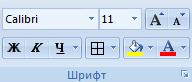
Change, for example, the font size, make the header “bold”. You can center the text, assign hyphens, etc.
How to create a table in Excel: step-by-step instructions
The simplest way to create tables is already known. But Excel has a more convenient option (in terms of subsequent formatting and working with data).
Let's make a “smart” (dynamic) table:

Note. You can take a different path - first select a range of cells, and then click the “Table” button.

Now enter the necessary data into the finished frame. If you need an additional column, place the cursor in the cell designated for the name. Enter the name and press ENTER. The range will automatically expand.

If you need to increase the number of lines, hook it in the lower right corner to the autofill marker and drag it down.
How to work with a table in Excel
With the release of new versions of the program, working with tables in Excel has become more interesting and dynamic. When a smart table is formed on a sheet, the “Working with Tables” - “Design” tool becomes available.
Here we can give the table a name and change its size.
Various styles are available, the ability to convert the table into a regular range or a summary report.
Features of dynamic MS Excel spreadsheets huge. Let's start with basic data entry and autofill skills:


If we click on the arrow to the right of each header subheading, we will get access to additional tools for working with table data.

Sometimes the user has to work with huge tables. To see the results, you need to scroll through more than one thousand lines. Deleting rows is not an option (the data will be needed later). But you can hide it. For this purpose, use numerical filters (picture above). Uncheck the boxes next to the values that should be hidden.
When the number of sheets in your book grows and navigation through it becomes problematic, I suggest creating a table of contents sheet for the book, with links to the necessary sheets.
insert a blank sheet into the book
in the “Insert Hyperlink” window, select what to link the hyperlink to: “Link to a place in the document.” Cell address - which cell of the sheet the cursor will be moved to. and select the place sheet Singapore. In the “Text” field, indicate the name of the sheet. After selecting the parameters, click OK.

The text in the cell has changed its appearance. This means that a hyperlink has been created for it. Let's set up hyperlinks to other sheets in the book in the same way. Please note that the hyperlink used to navigate changes its color. 
For convenience, you can also create backlinks on all sheets of your book, which will lead back to the table of contents. In order not to have to manually create hyperlinks and then copy them to each sheet, it is better to use another method - the HYPERLINK function.
We select all the sheets in the book where we want to add a back link (to mass select sheets, you need to hold down the Ctrl key and select the desired sheets with the mouse), and enter the following function in any suitable cell:
This function will create a hyperlink in the current cell on all selected sheets with the text “Back to Table of Contents”, clicking on which will return the user to the Table of Contents sheet.
How to create a button on a menu:
To make the menu more visually pleasing, let’s add buttons
First, let's create the shape of the future button: Insert → Shapes → Select any shape:

Let's print the text inside the shape. This is how we drew the button.
Select the shape → go to the Insert tab → Hyperlink. Next, assign parameters to it as in the first paragraph, and click OK. Similarly, you can create other hyperlink buttons on different sheets of the book. And add a little creativity using the FORMAT menu

If the number of sheets in your Excel workbook has exceeded the second ten, then navigating through the sheets begins to become a problem. One of the beautiful ways to solve this is to create a table of contents with hyperlinks leading to the corresponding sheets of the book:
There are several ways to implement this.
Video
Place in document
HYPERLINK Shift and/or Ctrl
Table of contents.
Open Name Manager on the tab Table of contents. In field Range (Reference) enter this formula:

GET.WORK.BOOK(1)
=GET.WORKBOOK(1)
Now in the variable Table of contents INDEX
Function ROW

REPLACE (SUBST) And FIND Name Manager from tab Table of contents and change its formula:

Table of contents Ctrl+Alt+F9
REPLACE(GET.WORKBOOK(1),1,FIND("]",GET.WORKBOOK(1));"") &T(TDATE())
Function TDATE (NOW) T TDATE
To hide errors #REFERENCE (#REF) INDEXIFERROR

HYPERLINK

Method 3. Macro
Method 2
Alt+F11 Insert - Module
Sub SheetList() Dim sheet As Worksheet Dim cell As Range With ActiveWorkbook For Each sheet In ActiveWorkbook.Worksheets Set cell = Worksheets(1).Cells(sheet.Index, 1) .Worksheets(1).Hyperlinks.Add anchor:=cell , Address:="", SubAddress:=""" & sheet.Name & """ & "!A1" cell.Formula = sheet.Name Next End With End Sub
Close the Visual Basic Editor and return to Excel. Add a blank sheet to the book and place it first. Then click Alt+F8 or open the menu SheetList
Method 1.
Related links
- What is a macro, how to create it, where to copy the text of the macro, how to run the macro?
- Automatically create a book table of contents with one button (PLEX Add-in)
- Sending emails using the HYPERLINK function
- Quickly switch between sheets in an Excel workbook
Method 1: Manually Created Hyperlinks
Insert a blank sheet into the workbook and add hyperlinks to the sheets you need using the command Insert - Hyperlink. In the window that opens, select the option on the left Place in document and set the external text display and the address of the cell where the link will lead:
For convenience, you can also create backlinks on all sheets of your book, which will lead back to the table of contents. In order not to have to manually create hyperlinks and then copy them to each sheet, it is better to use another method - the function HYPERLINK. We select all the sheets in the book where we want to add a backlink (you can use the keys to mass select sheets Shift and/or Ctrl) and in any suitable cell we enter a function of the following form:
This function will create a hyperlink in the current cell on all selected sheets with the text “Back to Table of Contents”, clicking on which will return the user to the sheet Table of contents.
Method 2: Dynamic table of contents using formulas
This, although slightly exotic, is a very beautiful and convenient way to create an automatic table of contents for your book. Exotic - because it uses an undocumented XLM feature GET.WORKBOOK, left by the developers for compatibility with older versions of Excel. This function dumps a list of all sheets in the current workbook into a given variable, from which we can then extract them and use them in our table of contents.
Open Name Manager on the tab Formulas (Formulas – Name Manager) and create a new named range called, let's say Table of contents. In field Range (Reference) enter this formula:
GET.WORK.BOOK(1)
=GET.WORKBOOK(1)
Now in the variable Table of contents contains our searched names. To extract them from there to the sheet, you can use the function INDEX, which “pulls out” elements from the array by their number:
Function ROW gives the current row number and, in this case, is needed only to avoid manually creating a separate column with the serial numbers of the elements being extracted (1,2,3...). Thus, in cell A1 we will have the name of the first sheet, in A2 - the name of the second, etc.
Not bad. However, as you can see, the function returns not only the sheet name, but also the workbook name, which we do not need. To remove it, we use the functions REPLACE (SUBST) And FIND, which will find the closing square bracket character (]) and replace all text up to and including that character with the empty string (""). Let's open it again Name Manager from tab Formulas (Formulas - Name Manager), double click to open the created range Table of contents and change its formula:
REPLACE(GET.WORKBOOK(1),1,FIND("]",GET.WORKBOOK(1));"")
=SUBST(GET.WORKBOOK(1);1;FIND("]";GET.WORKBOOK(1));"")
Now our list of sheets will look much better:
A small side complication is that our formula is in a named range Table of contents will be recalculated only when entered, or when the book is forced to recalculate by pressing a key combination Ctrl+Alt+F9. To get around this unpleasant moment, let’s add a small “tail” to our formula:
REPLACE(GET.WORKBOOK(1),1,FIND("]",GET.WORKBOOK(1));"") &T(TDATE())=SUBST(GET.WORKBOOK(1);1;FIND("]";GET.WORKBOOK(1));"")&T(NOW())
Function TDATE (NOW) gives the current date (with time), and the function T turns that date into an empty text string, which is then concatenated to our sheet name using the concatenation operator (&). Those. the sheet name does not actually change, but since the function TDATE is recalculated and produces a new time and date for any change in the sheet, then the rest of our formula will be forced to recalculate too and - as a result - the names of the sheets will be constantly updated.
To hide errors #REFERENCE (#REF), which will appear if we copy our formula with the function INDEX for more cells than we have sheets, we can use the function IFERROR, which catches any errors and replaces them with the empty string (""):
And finally, to add “live” hyperlinks to sheet names for quick navigation, you can use the same function HYPERLINK, which will form the address for the transition from the sheet name:
Method 3. Macro
And finally, you can use a simple macro to create a table of contents. True, you will have to run it every time the structure of the book changes - unlike Method 2, the macro itself does not track them.
Open the Visual Basic Editor by clicking Alt+F11 or by selecting (in older versions of Excel) from the menu Tools - Macro - Visual Basic Editor(Tools - Macro - Visual Basic Editor). In the editor window that opens, create a new empty module (menu Insert - Module ) and copy the text of this macro there:
Sub SheetList()
Dim sheet As Worksheet
Dim cell As Range
With ActiveWorkbook
For Each sheet In ActiveWorkbook.Worksheets
Set cell = Worksheets(1).Cells(sheet.Index, 1)
.Worksheets(1).Hyperlinks.Add anchor:=cell, Address:="", SubAddress:="'" & sheet.Name & "'" & "!A1"
cell.Formula = sheet.Name
Next
End With
End Sub Close the Visual Basic Editor and return to Excel. Add a blank sheet to the book and place it first. Then click Alt+F8 or open the menu Tools - Macro - Macros. Find the macro you created there SheetList and run it. The macro will create a list of hyperlinks with sheet names on the first sheet of the workbook. Clicking on any of them will take you to the desired sheet.
For convenience, you can also create backlinks on all sheets of your book, which will lead back to the table of contents, as described in Method 1.
My way. My version
T  Sheet name - =IFERROR(REPLACE(INDEX(Table of Contents,ROW()-3),1,FIND("]",INDEX(Table of Contents,ROW()-3));"");"")
Date - =IFERROR(IF(INDIRECT("'"&B4&"'"&"!A1″)=0;"";INDIRECT("'"&B4&"'"&"!A1″));"")
Name - =INDIRECT(“‘”&B4&”‘”&”!A3″)
PO - =INDIRECT(“‘”&B4&”‘”&”!E5″)
salary tax - =INDIRECT(“‘”&B4&”‘”&”!E6″)
depreciation - =INDIRECT(“‘”&B4&”‘”&”!E7″)
materials - =INDIRECT(“‘”&B4&”‘”&”!E8″)
vsp materials - =INDIRECT(“‘”&B4&”‘”&”!E9″)
INDIRECT("'"&B4&"'"&"!E10″)
INDIRECT("'"&B4&"'"&"!E11″)=INDIRECT("'"&B4&"'"&"!E12″)=INDIRECT("'"&B4&"'"&"!E13″)=INDIRECT( "'"&B4&"'"&"!E18″)=INDIRECT("'"&B4&"'"&"!E19″)
Download video and cut mp3 - we make it easy!
Our website is a great tool for entertainment and relaxation! You can always view and download online videos, funny videos, hidden camera videos, feature films, documentaries, amateur and home videos, music videos, videos about football, sports, accidents and disasters, humor, music, cartoons, anime, TV series and many other videos are completely free and without registration. Convert this video to mp3 and other formats: mp3, aac, m4a, ogg, wma, mp4, 3gp, avi, flv, mpg and wmv. Online Radio is a selection of radio stations by country, style and quality. Online Jokes are popular jokes to choose from by style. Cutting mp3 into ringtones online. Video converter to mp3 and other formats. Online Television - these are popular TV channels to choose from. TV channels are broadcast absolutely free in real time - broadcast online.